(To What is Chaos?)    (To Bifurcation Model)

Model: Logistic System (Xnext):
Time Series Diagrams

(Part 1 of 2 parts)

Strategies and Rubrics for Teaching Chaos and Complex Systems Theories as Elaborating, Self-Organizing, and Fractionating Evolutionary Systems,

Fichter, Lynn S., Pyle, E.J., and Whitmeyer, S.J., 2010, Journal of Geoscience Education (in press)

---

Description: We always begin with the logistic system, Xnext = rX (1-X). It is a simple population growth model that produces an 'S-shaped' "logistic" curve representing early exponential growth followed by stabilization (figures below). This can be considered one definition of chaos theory, or rather the behavior of the system is one definition of chaos theory (Gleick, 1988). This model usually takes an entire class, and we are more deliberate with developing it than many of the ideas that follow; likewise we will discuss this one more than the others.

      In the logistic system populations always range between 0.0 (extinction) and 1.0 (largest conceivable population). To ground the model, it is introduced as a population growth model—we talk about Gypsy moth infestations—and how we might use the model to make predictions about future population sizes. The growth of the population—the positive feedback—is the rX. The reversal of population growth—the negative feedback—is the (1-X). We also show a variety of logistic “S” curves garnered from the web to show how widely this model is used in many studies. This also demonstrates that the common, and not always correct understanding of the logistic system, is that it always does or should plot a diagnostic S-shaped curve.

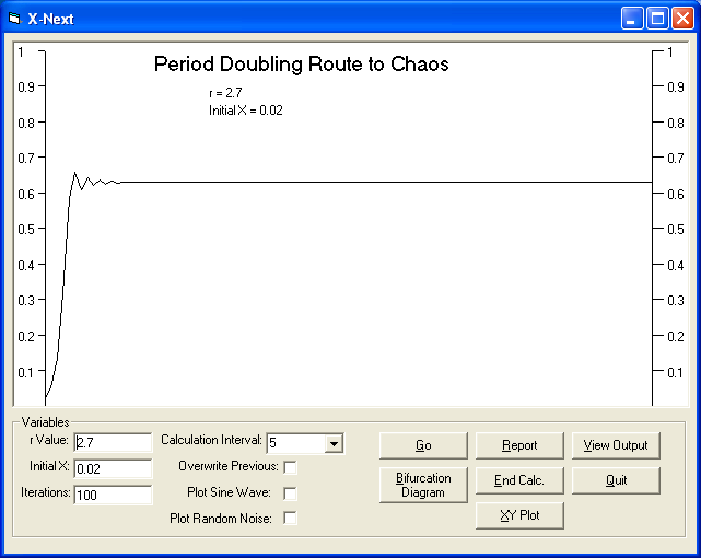
Presentation: After an introduction of general population growth models, we do one run through of the calculations by hand at an initial population of X=0.2 and ‘r’ value of 2.7. The rest of the calculations are done with a logistics program which plots out the population sizes changes on a time series diagram (Figure 1, and below).
     This is an interactive exercise between the students, the prof, and the model; i.e. we play a lot with the system, have fun with it, change parameters, experiment, debate with the students— just to see what happens.
      Initially, we run the model for 100 generations at 2.7 and ask the class to describe what they see; what happened. Next we ask for predictions of the behavior if we raise the ‘r’ value to 2.9, based on what they have just observed.
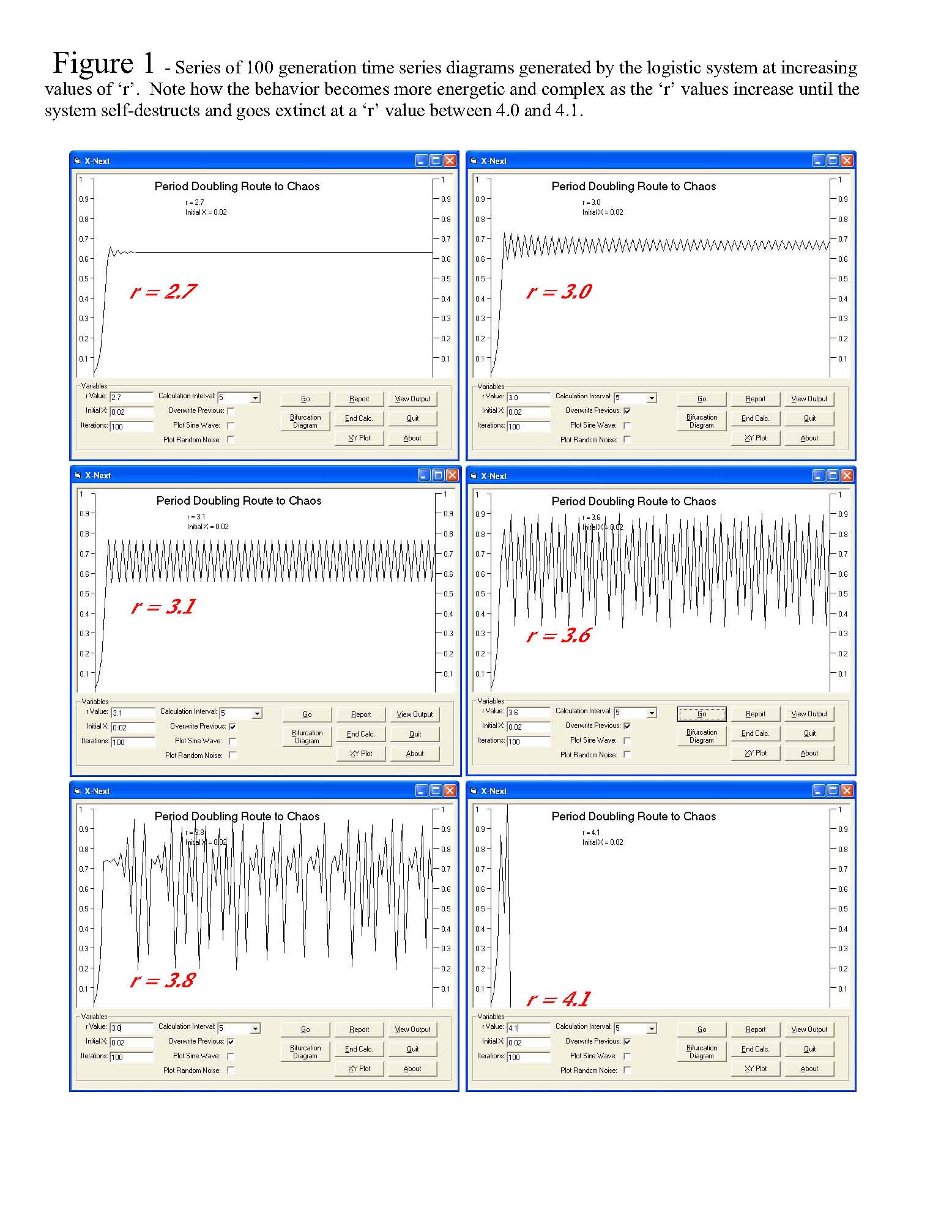
      This procedure is followed at increasing ‘r’ increments: 3.0, 3.1, 3.2 etc. until the system breaks at ‘r’ = < 4.1. The behavior evolves to amazing complexity. Figure 1 (below) shows the range of behavior over a range of ‘r’ values. At 2.7 the system attenuates to a single population size—a point attractor—at 3.1 it oscillates between two population sizes out to seven decimal places, but at 3.0 the question becomes, “Does it ever stop attenuating?” The answer is, “No” at least not to 1 million generations.
      We ask the class if they think it will ever attenuate at 3.0; how many generations they think it will take to find out; and run each of their suggestions to test their hypotheses. One other observation is to explore to how many decimal places the system has stabilized at each 'r' value; this gets to significant digits and how much precision a calculation needs to be to be useful.
     But, after each experiment we keep asking, “Ok, based on what you have observed so far, what do you want to do next; make a hypothesis.” This is that sense of interactive play.
      One of the other activities we have them do is to plot on a blank bifurcation diagram (see below) the final population sizes for each value of ‘r’ during the class discussion Go to: View Output. It helps to make the bifurcation diagram explored next easier to grasp.

Anticipated Learning Outcome:

1. Computational viewpoint: the idea that in a dynamic system the only way to know the outcome of an algorithm is to actually calculate it; there is no shorter route to knowing its behavior. This is not true at values below about 3.0, but becomes true at higher values. That this is not intuitively obvious is clear to the students because at higher ‘r’ values they are unable to predict the changing behavior of the system based on past behavior.

2. Positive/negative feedback: one central feature of all complex systems is that their behavior stems from the interplay of positive and negative feedbacks. This is a concept that students, when thrown into a natural complex system with many feedbacks operating, may have trouble grasping. The logistic system being so simple makes the influence of positive and negative feedback transparent.

3. ‘r’ values: ‘r’ can be translated as rate of growth, although we use ‘r’ from this point on to talk about whether the ‘r’ value of any system is high (dissipating lots of energy and/or information), or low (settling toward an equilibrium state).

4. Deterministic does not equal predictable: this is a very deep concept, especially if we explore its philosophical or theological roots (which in some classes we do). But, in classical science deterministic equals predictable, and predictable means it is deterministic. The logistic system is undeniably deterministic, but at higher ‘r’ values all semblance of predictability breaks down. For understanding complex systems this is the most important concept gained from exploration of the logistic system.

---

Power Point: Logistic System

Xnext - Logistic System - Computer Model

Msvbvm50.dll file some computers may require to make program active.

Bifurcation Diagram

- during class at each 'r' value we look at "View Output", check the last population sizes, and have them plot them on a bifurcation diagram (pdf version available by clicking image). This is preparation for the next demonstration.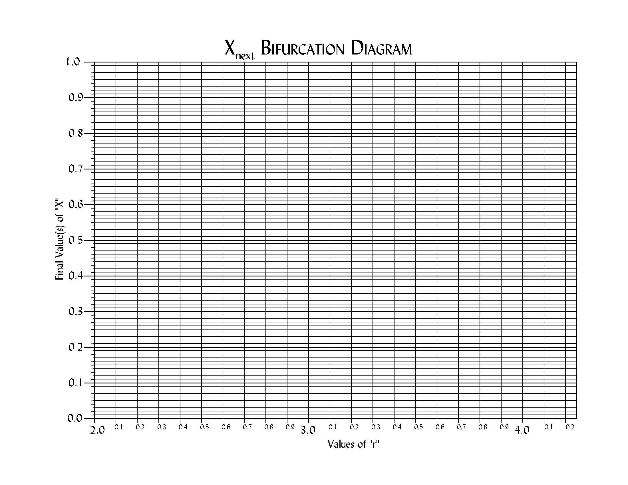

Figure 1

(To What is Chaos?)    (To Bifurcation Model)

---